How To Draw A Balance Scale

Imbalanced classes put "accuracy" out of business concern. This is a surprisingly common problem in machine learning (specifically in classification), occurring in datasets with a asymmetric ratio of observations in each grade.

Standard accuracy no longer reliably measures operation, which makes model training much trickier.

Imbalanced classes appear in many domains, including:

• Fraud detection
• Spam filtering
• Illness screening
• SaaS subscription churn
• Advertizement click-throughs

In this guide, we'll explore 5 effective ways to handle imbalanced classes.

Intuition: Illness Screening Case

Permit'due south say your client is a leading enquiry hospital, and they've asked you to train a model for detecting a affliction based on biological inputs nerveless from patients.

Merely hither'southward the grab… the disease is relatively rare; it occurs in just viii% of patients who are screened.

Now, before you fifty-fifty get-go, do you run across how the problem might break? Imagine if you didn't bother training a model at all. Instead, what if you but wrote a single line of lawmaking that always predicts 'No Affliction?'

def disease_screen ( patient_data ) : # Ignore patient_data render 'No Affliction.'

Well, guess what? Your "solution" would have 92% accurateness!

Unfortunately, that accuracy is misleading.

• For patients who practice not have the disease, yous'd have 100% accurateness.
• For patients whopractice have the disease, y'all'd have 0% accuracy.
• Your overall accuracy would be loftier simply because near patients do not have the affliction (not because your model is any good).

This is clearly a problem because many auto learning algorithms are designed to maximize overall accuracy. The rest of this guide volition illustrate different tactics for treatment imbalanced classes.

Of import notes before we brainstorm:

First, please note that we're not going to dissever out a dissever examination prepare, tune hyperparameters, or implement cross-validation. In other words, we're non necessarily going to follow all-time practices.

Instead, this tutorial is focused purely on addressing imbalanced classes.

In addition, not every technique below will work for every problem. However, 9 times out of 10, at to the lowest degree one of these techniques should do the fob.

Residue Scale Dataset

For this guide, we'll use a synthetic dataset called Balance Scale Data, which you can download from the UCI Machine Learning Repository here.

This dataset was originally generated to model psychological experiment results, merely it'southward useful for us because it's a manageable size and has imbalanced classes.

import pandas as pd import numpy equally np # Read dataset df = pd . read_csv ( 'rest-scale.data' , names=[ 'residue' , 'var1' , 'var2' , 'var3' , 'var4' ] ) # Display instance observations df . head ( )

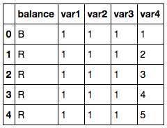
The dataset contains data about whether a scale is counterbalanced or not, based on weights and distances of the two artillery.

• It has ane target variable, which nosotros've labeled residuum  .
• It has 4 input features, which we've labeled var1   through var4  .

The target variable has three classes.

• R for right-heavy, i.eastward. when var3 * var4 > var1 * var2
• L for left-heavy, i.eastward. when var3 * var4 < var1 * var2
• B for balanced, i.e. when var3 * var4 = var1 * var2

df [ 'rest' ] . value_counts ( ) # R    288 # L    288 # B     49 # Proper name: rest, dtype: int64

However, for this tutorial, we're going to plow this into a binary nomenclature problem.

Nosotros're going to label each observation as1 (positive grade) if the scale is balanced or0 (negative course) if the calibration is not balanced:

# Transform into binary nomenclature df [ 'balance' ] = [ 1 if b=='B' else 0 for b in df . residuum ] df [ 'balance' ] . value_counts ( ) # 0    576 # i     49 # Proper name: residual, dtype: int64 # Nearly viii% were balanced

Every bit you can run into, only nigh 8% of the observations were counterbalanced. Therefore, if we were to e'er predict0, we'd accomplish an accuracy of 92%.

The Danger of Imbalanced Classes

Now that we have a dataset, nosotros can really show the dangers of imbalanced classes.

Kickoff, let'due south import the Logistic Regression algorithm and the accurateness metric from Scikit-Learn.

from sklearn . linear_model import LogisticRegression from sklearn . metrics import accuracy_score

Next, we'll fit a very simple model using default settings for everything.

# Divide input features (10) and target variable (y) y = df . balance X = df . drop ( 'balance' , axis=ane ) # Train model clf_0 = LogisticRegression ( ) . fit ( 10 , y ) # Predict on training set pred_y_0 = clf_0 . predict ( X )

As mentioned above, many machine learning algorithms are designed to maximize overall accuracy by default.

We can confirm this:

# How's the accuracy? impress ( accuracy_score ( pred_y_0 , y ) ) # 0.9216

So our model has 92% overall accuracy, but is it because it's predicting only 1 class?

# Should nosotros be excited? print ( np . unique ( pred_y_0 ) ) # [0]

As you tin see, this model is just predicting0, which ways it'south completely ignoring the minority class in favor of the majority class.

Adjacent, nosotros'll look at the showtime technique for handling imbalanced classes: upwards-sampling the minority grade.

ane. Up-sample Minority Class

Upwards-sampling is the process of randomly duplicating observations from the minority course in order to reinforce its betoken.

In that location are several heuristics for doing and so, merely the near common way is to only resample with replacement.

First, we'll import the resampling module from Scikit-Learn:

from sklearn . utils import resample

Side by side, we'll create a new DataFrame with an upwards-sampled minority class. Here are the steps:

1. Get-go, we'll separate observations from each class into unlike DataFrames.
2. Adjacent, we'll resample the minority class with replacement, setting the number of samples to match that of the bulk grade.
3. Finally, we'll combine the up-sampled minority course DataFrame with the original majority class DataFrame.

Here's the code:

i ii 3 4 5 6 7 eight 9 10 11 12 13 14 fifteen xvi 17 18

# Split majority and minority classes df_majority = df [ df . balance==0 ] df_minority = df [ df . residual==i ] # Upsample minority course df_minority_upsampled = resample ( df_minority , replace=True , # sample with replacement n_samples=576 , # to match majority class random_state=123 ) # reproducible results # Combine majority class with upsampled minority class df_upsampled = pd . concat ( [ df_majority , df_minority_upsampled ] ) # Brandish new class counts df_upsampled . balance . value_counts ( ) # 1    576 # 0    576 # Name: balance, dtype: int64

Every bit you can see, the new DataFrame has more observations than the original, and the ratio of the 2 classes is now 1:1.

Let's railroad train some other model using Logistic Regression, this fourth dimension on the balanced dataset:

one two 3 4 v half-dozen 7 8 9 ten eleven 12 13 14 15 16 17

# Separate input features (X) and target variable (y) y = df_upsampled . balance X = df_upsampled . drib ( 'balance' , axis=1 ) # Railroad train model clf_1 = LogisticRegression ( ) . fit ( 10 , y ) # Predict on preparation set pred_y_1 = clf_1 . predict ( Ten ) # Is our model still predicting just one grade? print ( np . unique ( pred_y_1 ) ) # [0 1] # How'south our accuracy? impress ( accuracy_score ( y , pred_y_1 ) ) # 0.513888888889

Bully, now the model is no longer predicting just one class. While the accuracy also took a nosedive, information technology'due south now more meaningful every bit a performance metric.

2. Downwards-sample Bulk Class

Down-sampling involves randomly removing observations from the bulk course to prevent its signal from dominating the learning algorithm.

The almost mutual heuristic for doing so is resampling without replacement.

The process is like to that of upward-sampling. Hither are the steps:

1. First, we'll carve up observations from each course into different DataFrames.
2. Adjacent, nosotros'll resample the majority class without replacement, setting the number of samples to friction match that of the minority class.
3. Finally, we'll combine the down-sampled bulk class DataFrame with the original minority class DataFrame.

Here's the lawmaking:

1 2 three 4 five vi 7 eight nine ten eleven 12 13 xiv 15 xvi 17 18

# Separate majority and minority classes df_majority = df [ df . balance==0 ] df_minority = df [ df . balance==ane ] # Downsample majority grade df_majority_downsampled = resample ( df_majority , replace=False , # sample without replacement n_samples=49 , # to match minority course random_state=123 ) # reproducible results # Combine minority class with downsampled majority class df_downsampled = pd . concat ( [ df_majority_downsampled , df_minority ] ) # Brandish new grade counts df_downsampled . residue . value_counts ( ) # ane    49 # 0    49 # Name: balance, dtype: int64

This time, the new DataFrame has fewer observations than the original, and the ratio of the two classes is at present one:1.

Over again, let'due south railroad train a model using Logistic Regression:

1 two 3 iv five 6 seven 8 9 ten 11 12 13 xiv xv 16 17

# Separate input features (X) and target variable (y) y = df_downsampled . balance 10 = df_downsampled . drop ( 'residue' , axis=1 ) # Train model clf_2 = LogisticRegression ( ) . fit ( X , y ) # Predict on training fix pred_y_2 = clf_2 . predict ( 10 ) # Is our model still predicting only 1 class? impress ( np . unique ( pred_y_2 ) ) # [0 one] # How's our accuracy? print ( accuracy_score ( y , pred_y_2 ) ) # 0.581632653061

The model isn't predicting just 1 grade, and the accuracy seems college.

We'd all the same want to validate the model on an unseen test dataset, but the results are more than encouraging.

3. Alter Your Performance Metric

And then far, we've looked at two ways of addressing imbalanced classes past resampling the dataset. Next, nosotros'll expect at using other operation metrics for evaluating the models.

Albert Einstein in one case said, "if you approximate a fish on its ability to climb a tree, it will alive its whole life believing that it is stupid." This quote really highlights the importance of choosing the right evaluation metric.

For a full general-purpose metric for classification, nosotros recommendArea Under ROC Curve (AUROC).

• We won't dive into its details in this guide, but you tin can read more about information technology here.
• Intuitively, AUROC represents the likelihood of your model distinguishing observations from two classes.
• In other words, if you randomly select one observation from each class, what'south the probability that your model will exist able to "rank" them correctly?

We can import this metric from Scikit-Acquire:

from sklearn . metrics import roc_auc_score

To calculate AUROC, you lot'll demand predicted class probabilities instead of just the predicted classes. You can get them using the . predict_proba ( ) function like so:

# Predict class probabilities prob_y_2 = clf_2 . predict_proba ( Ten ) # Keep just the positive class prob_y_2 = [ p [ 1 ] for p in prob_y_2 ] prob_y_2 [ : 5 ] # Example # [0.45419197226479618, #  0.48205962213283882, #  0.46862327066392456, #  0.47868378832689096, #  0.58143856820159667]

And then how did this model (trained on the downwards-sampled dataset) practise in terms of AUROC?

impress ( roc_auc_score ( y , prob_y_2 ) ) # 0.568096626406

Ok... and how does this compare to the original model trained on the imbalanced dataset?

prob_y_0 = clf_0 . predict_proba ( Ten ) prob_y_0 = [ p [ i ] for p in prob_y_0 ] print ( roc_auc_score ( y , prob_y_0 ) ) # 0.530718537415

Call up, our original model trained on the imbalanced dataset had an accuracy of 92%, which is much college than the 58% accuracy of the model trained on the down-sampled dataset.

However, the latter model has an AUROC of 57%, which is higher than the 53% of the original model (but not by much).

Note: if you got an AUROC of 0.47, it just means you demand to capsize the predictions considering Scikit-Larn is misinterpreting the positive class. AUROC should be >= 0.five.

4. Penalize Algorithms (Cost-Sensitive Training)

The next tactic is to employ penalized learning algorithms that increase the cost of classification mistakes on the minority course.

A popular algorithm for this technique is Penalized-SVM:

from sklearn . svm import SVC

During training, nosotros can use the statement class_weight='counterbalanced'   to penalize mistakes on the minority grade by an amount proportional to how under-represented information technology is.

We also want to include the argument probability=True   if nosotros desire to enable probability estimates for SVM algorithms.

Let'due south train a model using Penalized-SVM on the original imbalanced dataset:

1 2 iii iv 5 6 seven viii 9 10 11 12 13 14 15 16 17 18 19 20 21 22 23 24 25 26 27

# Separate input features (Ten) and target variable (y) y = df . residue X = df . drop ( 'balance' , axis=1 ) # Railroad train model clf_3 = SVC ( kernel='linear' , class_weight='counterbalanced' , # penalize probability=True ) clf_3 . fit ( X , y ) # Predict on training set pred_y_3 = clf_3 . predict ( Ten ) # Is our model still predicting simply one form? print ( np . unique ( pred_y_3 ) ) # [0 ane] # How's our accuracy? print ( accuracy_score ( y , pred_y_3 ) ) # 0.688 # What about AUROC? prob_y_3 = clf_3 . predict_proba ( X ) prob_y_3 = [ p [ 1 ] for p in prob_y_3 ] impress ( roc_auc_score ( y , prob_y_3 ) ) # 0.5305236678

Once again, our purpose here is only to illustrate this technique. To really make up one's mind which of these tactics works best for this problem, you'd want to evaluate the models on a concur-out exam set.

five. Apply Tree-Based Algorithms

The final tactic we'll consider is using tree-based algorithms. Decision copse often perform well on imbalanced datasets because their hierarchical structure allows them to learn signals from both classes.

In modern applied machine learning, tree ensembles (Random Forests, Slope Boosted Copse, etc.) almost always outperform singular decision copse, and then nosotros'll jump right into those:

from sklearn . ensemble import RandomForestClassifier

At present, permit's train a model using a Random Forest on the original imbalanced dataset.

ane ii 3 4 5 half-dozen seven 8 nine x eleven 12 13 xiv 15 16 17 xviii 19 twenty 21 22 23 24

# Carve up input features (X) and target variable (y) y = df . rest X = df . drop ( 'balance' , axis=1 ) # Train model clf_4 = RandomForestClassifier ( ) clf_4 . fit ( X , y ) # Predict on preparation set pred_y_4 = clf_4 . predict ( X ) # Is our model still predicting merely one class? print ( np . unique ( pred_y_4 ) ) # [0 1] # How's our accuracy? print ( accuracy_score ( y , pred_y_4 ) ) # 0.9744 # What about AUROC? prob_y_4 = clf_4 . predict_proba ( X ) prob_y_4 = [ p [ 1 ] for p in prob_y_4 ] print ( roc_auc_score ( y , prob_y_4 ) ) # 0.999078798186

Wow! 97% accuracy and about 100% AUROC? Is this magic? A sleight of paw? Cheating? Likewise good to be truthful?

Well, tree ensembles take become very popular considering they perform extremely well on many real-world issues. We certainly recommend them wholeheartedly.

However:

While these results are encouraging, the modelcould be overfit, so you should nonetheless evaluate your model on an unseen test set earlier making the final decision.

Annotation: your numbers may differ slightly due to the randomness in the algorithm. You can fix a random seed for reproducible results.

Honorable Mentions

There were a few tactics that didn't get in into this tutorial:

Create Synthetic Samples (Data Augmentation)

Creating constructed samples is a shut cousin of upward-sampling, and some people might categorize them together. For example, the SMOTE algorithm is a method of resampling from the minority class while slightly perturbing feature values, thereby creating "new" samples.

You can discover an implementation of SMOTE in the imblearn library.

Combine Minority Classes

Combining minority classes of your target variable may be advisable for some multi-form issues.

For instance, let's say you wished to predict credit carte fraud. In your dataset, each method of fraud may be labeled separately, merely you might non intendance about distinguishing them. You could combine them all into a single 'Fraud' grade and care for the problem as binary nomenclature.

Reframe as Anomaly Detection

Anomaly detection, a.k.a. outlier detection, is for detecting outliers and rare events. Instead of edifice a nomenclature model, yous'd take a "profile" of a normal ascertainment. If a new observation strays likewise far from that "normal profile," information technology would be flagged equally an anomaly.

Determination & Next Steps

In this guide, we covered 5 tactics for handling imbalanced classes in machine learning:

1. Up-sample the minority grade
2. Downward-sample the majority class
3. Change your performance metric
4. Penalize algorithms (cost-sensitive grooming)
5. Utilise tree-based algorithms

These tactics are subject to the No Complimentary Lunch theorem, and you should attempt several of them and apply the results from the examination ready to determine on the best solution for your problem.

Source: https://elitedatascience.com/imbalanced-classes

Posted by: leveyoverects36.blogspot.com

Share this post